rlauxe
rlauxe (“r-lux”)
WORK IN PROGRESS last changed: 02/17/2026
A library for Risk Limiting Audits (RLA), based on Philip Stark’s SHANGRLA framework and related code. The Rlauxe library is an independent implementation of the SHANGRLA framework, based on the published papers of Stark et al.
The SHANGRLA python library is the work of Philip Stark and collaborators, released under the AGPL-3.0 license.
Rlauxe uses the Raire Java library for Ranked Choice contests, also called Instant runoff Voting (IRV). Raire-Java is Copyright 2023-2025 Democracy Developers. It is based on software (c) Michelle Blom in C++ https://github.com/michelleblom/audit-irv-cp/tree/raire-branch, and released under the GNU General Public License v3.0.
Click on plot images to get an interactive html plot. You can also read this document on github.io.
Table of Contents
- SHANGRLA framework
- Rlauxe Workflow Overview
- Audit Types
- Comparing Sample Sizes by Audit type
- Estimating Sample Batch sizes
- Multiple Contest Auditing
- Reference Papers
- Appendices
SHANGRLA framework
SHANGRLA is a framework for running Risk Limiting Audits for elections. It uses a statistical risk testing function that allows an audit to statistically prove that an election outcome is correct (or not) to within a risk level α. For example, a risk limit of 5% means that the election outcome (i.e. the winner(s)) is correct with 95% probability.
It uses an assorter to assign a number to each ballot, and checks outcomes by testing half-average assertions, each of which claims that the mean of a finite list of numbers is greater than 1/2. The complementary null hypothesis is that the assorter mean is not greater than 1/2. If that hypothesis is rejected for every assertion, the audit concludes that the outcome is correct. Otherwise, the audit expands, potentially to a full hand count. If every assertion is tested at risk level α, this results in a risk-limiting audit with risk limit α: if the election outcome is not correct, the chance the audit will stop shy of a full hand count is at most α.
| term | definition |
|---|---|
| audit | iterative process of choosing ballots and checking if all the assertions are true. |
| risk | we want to confirm or reject with risk level α. |
| assorter | assigns a number between 0 and upper to each card, chosen to make assertions “half average”. |
| assertion | the mean of assorter values is > 1/2: “half-average assertion” |
| bettingFn | decides how much to bet for each sample. (BettingMart) |
| riskFn | the statistical method to test if the assertion is true. |
| Nc | a trusted, independent bound on the number of valid cards cast in the contest c. |
| Ncast | the number of cards validly cast in the contest |
| Npop | the number of cards that might contain the contest |
Rlauxe Workflow Overview
1.Before the Audit
For each contest:
- Describe the contest name, candidates, contest type (eg Plurality), etc in the ContestInfo.
- Count the votes in the usual way. The reported winner(s) and the reported margins are based on this vote count.
- Determine the total number of valid cards (Nc), and number of votes cast (Ncast) for the contest.
- The software generates the assertions needed to prove (or not) that the winners are correct.
- Write the ContestWithAssertions to contests.json file
Create the Card Manifest:
- Create a Card Manifest, in which every physical card has a unique entry (called the AuditableCard).
- If this is a CLCA, attach the Cast Vote Record (CVR) from the vote tabulation system, to its AuditableCard.
- Optionally create Populations (eg OneAudit Pools) that describe each unique “population” of cards, and which contests are contained in the population. Cards that do not have complete CVRs should reference the population they are contained in.
- The Card Manifest is the ordered list of AuditableCards.
- Write the Card Manifest to cardManifest.csv, and optionally the Populations to populations.json.
Committment:
- Write the contests.json, populations.json, and cardManifest.csv files to a publically accessible “bulletin board”.
- Digitally sign these files; they constitute the “audit committment” and may not be altered once the seed is chosen.
2.Creating a random seed
- Create a random 32-bit integer “seed” in a way that allows public observers to be confident that it is truly random.
- Publish the random seed to the bulletin board. It becomes part of the “audit committment” and may not be altered once chosen.
- Use a PRNG (Psuedo Random Number Generator) with the random seed, and assign the generated PRNs, in order, to the auditable cards.
- Sort the cards by PRN and write them to sortedCards.csv.
3.Starting the Audit
The Election Auditors (EA) can examine the audit committment files, run simulations to estimate how many cards will need to be sampled, etc. The EA can choose:
- which contests will be included in the Audit
- the risk limit
- other audit configuration parameters
The audit configuration parameters are written to auditConfig.json.
4.Audit Rounds
The audit proceeds in rounds:
- Estimation: for each contest, estimate how many samples are needed to satisfy the risk limit
- Choosing contests and sample sizes: the EA decides which contests and how many samples will be audited. This may be done with an automated algorithm, or the Auditor may make individual contest choices.
- Random sampling: The actual ballots to be sampled are selected in order from the sorted Card Manifest until the sample size is satisfied.
- Manual Audit: find the chosen paper ballots that were selected to audit and do a manual audit of each.
- Create MVRs: enter the results of the manual audits (as Manual Vote Records, MVRs) into the system.
- Run the audit: For each contest, using the MVRs, calculate if the risk limit is satisfied.
- Decide on Next Round: for each contest not satisfied, decide whether to continue to another round, or call for a hand recount.
Each round generates samplePrns.json, sampleCards.csv, sampleMvrs.csv, and auditState.json files, which become part of the Audit Record.
5.Verification
Independently written verifiers can read the Audit Record and verify that the audit was correctly performed. See Verification.
Audit Types
In all cases:
- There must be a Card Location Manifest defining the population of ballots, that contains a unique identifier or location description that can be used to find the corresponding physical ballot.
- For each contest, there must be an independently determined upper bound on the number of cast cards/ballots that contain the contest.
Card Level Comparison Audits (CLCA)
When the election system produces an electronic record for each ballot card, known as a Cast Vote Record (CVR), then Card Level Comparison Audits can be done that compare sampled CVRs with the corresponding hand audited ballot card, known as the Manual Vote Record (MVR). A CLCA typically needs many fewer sampled ballots to validate contest results than other methods.
The requirements for CLCA audits:
- The election system must be able to generate machine-readable Cast Vote Records (CVRs) for each ballot.
- Unique identifiers must be assigned to each physical ballot, and recorded on the CVR, in order to find the physical ballot that matches the sampled CVR.
For the risk function, rlauxe uses the BettingMart function with the GeneralAdaptiveBetting betting function. GeneralAdaptiveBetting uses estimates/measurements of the error rates between the Cvrs and the Mvrs. If the error estimates are correct, one gets optimal “sample sizes”, the number of ballots needed to prove the election is correct.
See Betting risk function for overview of the risk and betting functions.
OneAudit CLCA
OneAudit is a type of CLCA audit, based on the ideas and mathematics of the ONEAudit papers (see appendix). It deals with the cases where:
- CVRS are not available for all ballots, and the remaining ballots are in one or more “pools” for which subtotals are available. (This is the Boulder “redacted votes” case.)
- CVRS are available for all ballots, but some cannot be matched to physical ballots. (This is the San Francisco case where mail-in ballots have matched CVRS, and in-person precinct votes have unmatched CVRs. Each precinct’s ballots are kept in a separate pool.)
In both cases we create an “overstatement-net-equivalent” (ONE) CVR for each pool, and use the average assorter value in that pool as the value of the (missing) CVR in the CLCA overstatement. When a ballot has been chosen for hand audit:
- If it has a CVR, use the standard CLCA over-statement assorter.
- If it has no CVR, use the overstatement-net-equivalent (ONE) CVR from the pool that it belongs to.
Thus, all cards must either have a CVR or be contained in a pool.
See Betting with OneAudit Pools for overview of OneAudit betting.
For details of OneAudit use cases, see OneAudit Use Cases.
Polling Audits
When CVRs are not available, a Polling audit can be done instead. A Polling audit
creates an MVR for each ballot card selected for sampling, just as with a CLCA, except without the CVR.
For the risk function, Rlaux uses the AlphaMart risk function with the ShrinkTrunkage estimation of the true population mean.
Comparing Sample Sizes by Audit type
In this section we characterize the number of samples needed for each audit type. For clarity of presentaton, we assume we have only one contest, and also ignore the need to estimate a batch size for each audit round. This is called a “one sample at a time” audit, which terminates as soon as the risk limit is confirmed or rejected.
In the section Estimating Sample Batch sizes below, we deal with the need to estimate a batch size, and the extra overhead of audit rounds. In the section Multiple Contest Auditing below, we deal with the complexity of having multiple contests on ballots.
In general, samplesNeeded is independent of the population size N. Rather, samplesNeeded depends on the diluted margin as well as the random sequence of ballots chosen to be hand audited.
(Actually there is a slight dependence on N for “without replacement” audits when the sample size approaches N, but that case approaches a full hand audit, and isnt very interesting.)
The following plots are simulations, averaging the results from the stated number of runs.
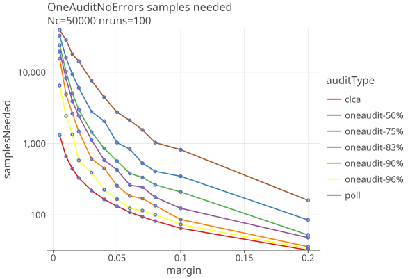
Samples needed with no errors
The audit type needing the least samples is CLCA when there are no errors in the CVRs, and no phantom ballots. In that case, the samplesNeeded depend only on the margin, and is a straight line vs margin on a log-log plot.
The smallest sample size for CLCA when there are no errors is when you always bet the maximum (1/µ_i, approximately 2). However, if there are errors and the assort value is 0.0, the maximum bet will “stall” the audit and the audit cant recover (see details). To avoid this, rlauxe limits how close the bet can be to the maximum. Here is a plot of CLCA no-error audits with the bet limited to 70, 80, 90, and 100% of the maximum:

We call this bet limit the “maximum risk”, expressed as a percent of the maximum bet. At any setting of maximum risk, the CLCA assort value is always the same when there are no errors, and so there is no variance: the plot above shows the exact numebr of samples needed as a function of margin and maximum risk.
For polling, the assort values vary, and the number of samples needed depends on the order the samples are drawn. Here we show the average and standard deviation over 100 independent trials at each reported margin, when no errors are found:

For OneAudit, results depend on the percent of CVRs vs pooled data, the pool averages and if there are multiple card styles in the pools. The following is a best case scenario with no errors in the CVRs, a single pool with the same margin and a single card style, with several values of the CVR percentage, as a function of margin, and maxRisk = .9:
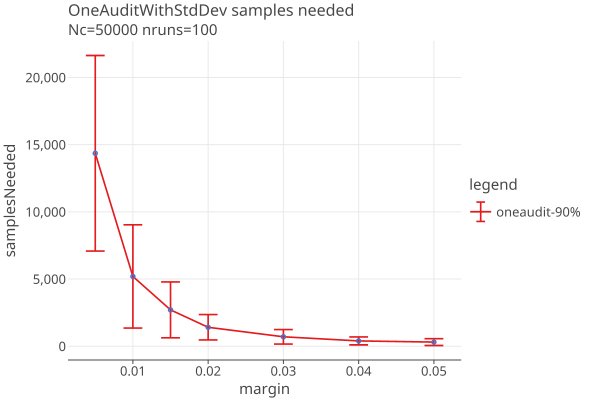
However, OneAudit has a large variance due to the random sequence of pool values. Here are the one sigma intervals for a “best case” 90% CVR OneAudit (for example, a 2% margin contest has a one-sigma interval of (466, 2520), click on the image to get an interactive plot):
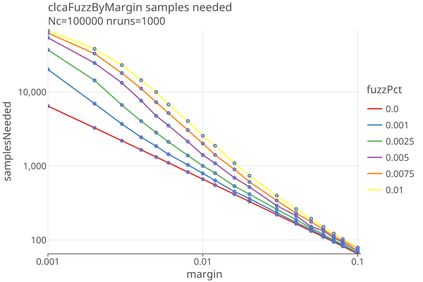
Samples needed when there are errors
In the following simulations, errors are created between the CVRs and the MVRs, by taking fuzzPct of the cards and randomly changing the candidate that was voted for. When fuzzPct = 0.0, the CVRs and MVRs agree. When fuzzPct = 0.01, 1% of the contest’s votes were randomly changed, and so on.
This fuzzing mechanism is rather crude, and may not reflect any real-world pattern of errors. See ClcaErrors for a deeper understanding of the effect of CLCA errors.
CLCA with errors
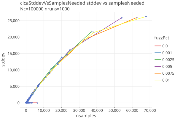
Here are the results of 1000 simulations of CLCA average samplesNeeded by margin for various values of fuzzPct:
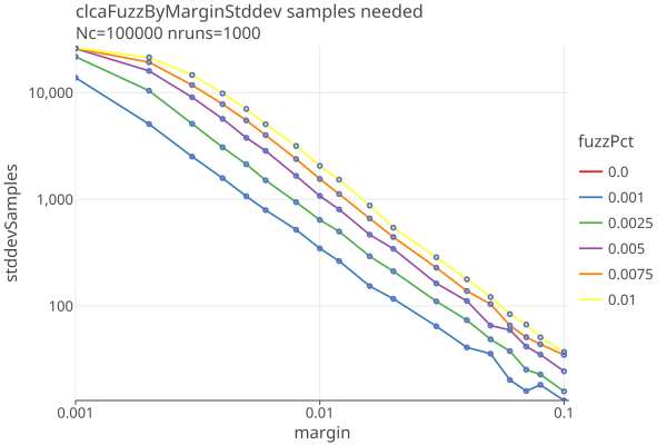
The average samplesNeeded dont tell the whole picture. There is a distribution of samplesNeeded whose variance is roughly proportional to the samplesNeeded; here is the standard deviation of those distributions with dependence on margin and fuzzPct:
A plot of standard deviation against samples needed shows an approximate linear relationship, approximately independent of fuzzPct when nsamples < 30,000:
A straight line implies
stddev = b + m * nsamples
where m is the slope of the line. We will take representative points (x0 = 68, y0 = 16) and (x1 = 37028, y1 = 21675)
m = (y2 - y1) / (x2 - x1)
  = (21675 - 16) / (37028 - 68)
  = .586

stddev = b + m * nsamples
b = stddev - m * nsamples
b = y0 - m * x0
b = 16 - .586 * 68
b = -23.85
so our approximate fit is:
stddev = .586 * nsamples - 23.85
which we show on a log-log plot here:
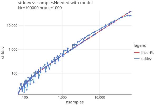
These results are generated by our single round (no estimation phase) CLCA algorithm with maxRisk = .9, and would be different with other choices of algorithm parameters.
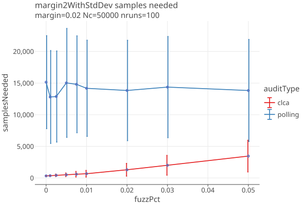
Comparison of CLCA, Polling, and OneAudit
With the margin fixed at 2%, this plot compares polling and CLCA audits and their variance:
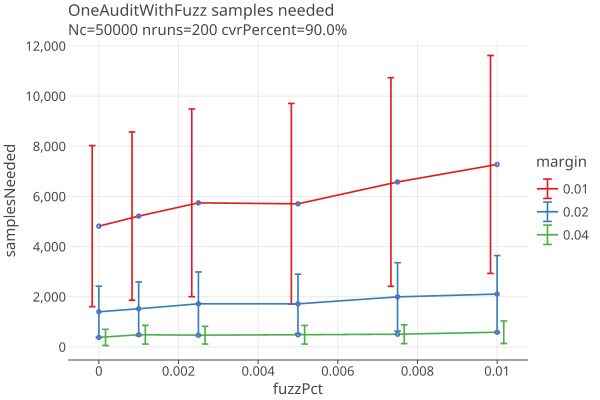
Here are just CLCA audits with margins of .01, .02, and .04, over a range of fuzz errors from 0 to 1%:

- Polling audit sample sizes are all but impervious to errors, because the sample variance dominates the errors.
- As margins get smaller, the variance in CLCA audits increases. At .001 fuzz (1 in 1000), an audit with a margin of 1% has an average sample size of 814, but the 1-sigma range goes from 472 to 1157.
- A rule of thumb might be that if you want to do CLCA audits down to 1% margin, your error rate must be less than 1/1000.
Here are similar results for OneAudits with fuzz in their CVRs:
We dont see that much change as the CLCA errors increase; the variance generated by the CLCA errors is small compared to the OneAudit variance from the pooled data.
Effect of Phantoms on Samples needed
Varying phantom percent, up to and over the margin of 4.5%, with errors generated with 1% fuzz:
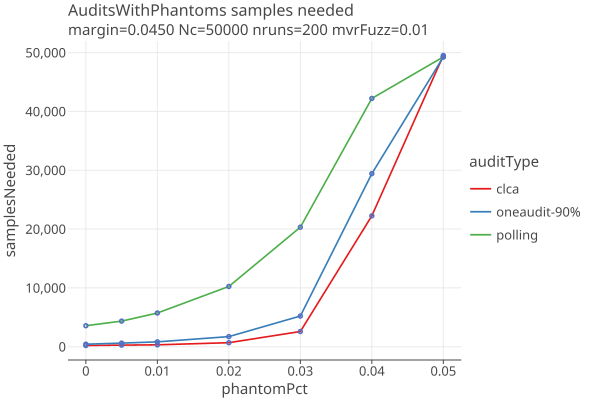
- Increased phantoms have a strong effect on sample size.
- All audits go to hand count when phantomPct gets close to the margin, as they should.
- See effect of Phantoms on samples needed that shows how many extra ballots are needed when a phantom ballot is sampled.
Estimating Sample Batch sizes
Sampling refers to choosing which ballots to hand review to create Manual Voting Records (MVRs). Once the ballots are located and the MVRs created, the actual audit takes place.
Audits are done in rounds. The auditors must decide how many cards/ballots they are willing to audit, since at some point its more efficient to do a full handcount than the more elaborate process of tracking down ballots that have been randomly selected for the sample.
Theres a tradeoff between the overall number of ballots sampled and the number of rounds. But we would like to minimize both.
Note that in this section we are plotting nmvrs = overall number of ballots sampled, which includes the inaccuracies of the estimation. Above we have been plotting samples needed, as if we were doing “one ballot at a time” auditing.
There are two phases to sampling: estimating the sample batch sizes for each contest, and then choosing ballots that contain at least that many contests in the canonical random ordering.
Estimation
For each contest we simulate the audit with manufactured data that has the same margin as the reported outcome, and a guess at the error rates.
For each contest assertion we run auditConfig.nsimEst (default 100) simulations and collect the distribution of samples needed to satisfy the risk limit. We then choose the (auditConfig.quantile) sample size as our estimate for that assertion. The contest’s estimated sample size is the maximum over the contest’s assertions.
If the simulation is accurate, the audit should succeed auditConfig.quantile fraction of the time (default 80%). Since we dont know the actual error rates, or the order that the errors will be sampled, these simulation results are just estimates.
Choosing ballots
Once we have all of the contests’ estimated sample sizes, we next choose which ballots/cards to sample. This step depends on the CardManifest and Population information, which tells which cards may have which contests. The number of cards that may have a contest on it is called the contests’s population size (Npop) and is used as the denominator of the diluted margin for the contest. The sampling must be uniform over the contest’s populations for a statistically valid audit.
The Population objects are a generalization of SHANGRLA’s Card Style Data, allowing for partial information about which cards have which contests. When you know exactly what contests are on each card, the diluted margin is at a maximum, and the samples needed is at a minimum. If you dont know exactly what contests are on each card, the cards may be divided up into populations in a way that minimizes the number of cards that might have the contest. See SamplePopulations for more explanation and current thinking.
For CLCA audits, the generated Cast Vote Records (CVRs) tell you exactly which cards have which contests, as long as the CVR records the undervotes (contests where no vote was cast). For Polling audits and OneAudit pools (and the case where cvrsContainUndervotes = false), the Populations describe which contests may be on which cards.
Note that each round does its own sampling without regard to the previous round’s results. However, since the seed remains the same, the ballot ordering is the same throughout the audit. We choose the lowest ordered ballots first, so previously audited MVRS are always used again in subsequent rounds, for contests that continue to the next round.
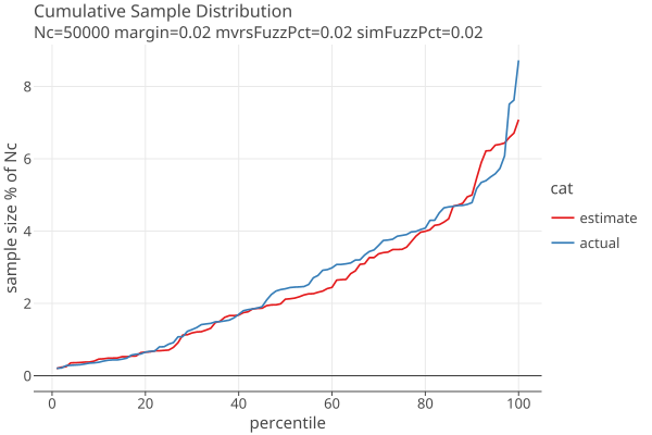
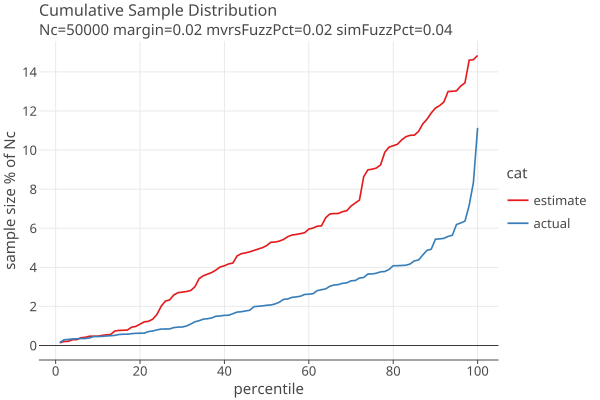
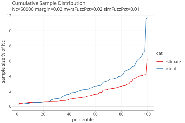
Under/Over estimating CLCA sample sizes
Overestimating sample sizes uses more hand-counted MVRs than needed. Underestimating sample sizes forces more rounds than needed. Over/under estimation is strongly influenced by over/under estimating error rates.
The following plots show approximate distribution of estimated and actual sample sizes, using our standard betting function with weight parameter d = 100, for margin=2% and errors in the MVRs generated with 2% fuzz.
When the estimated error rates are equal to the actual error rates:
When the estimated error rates are double the actual error rates:
When the estimated error rates are half the actual error rates:
These are generated without using rounds. When using rounds, surprisingly its better to start with an initial guess of no simulated fuzzing, as these plots show:
Here are the average extra samples vs the average number of rounds for mvrs with 1/1000 fuzz:


Here are the average extra samples vs the average number of rounds for mvrs with 2/1000 fuzz:


Here are the average extra samples vs the average number of rounds for mvrs with 3/1000 fuzz:


In all three cases, using 0% simulation has the lowest extra samples, better than using simFuzzPct that matches the true fuzz (fuzzMvrs). Note that these are averages over 1000 trials. The reason is probably that with a large variance, one is better off underestimating the sample size on the first round, and then on the second round using the measured error rates to estimate how many are left to do.
And trade off is that the average number of rounds goes up.
Based on these finding, we designed the “optimistic” strategy, which uses the calculated number of samples needed if there are no errors, for round 1. For subsequent rounds, it uses the measured error rates from round 1 to simulate a distribution, and takes auditConfig.quantile (default 80%) percentile as its estimate. The results of this strategy are shown here:


Here are the average extra samples vs the average number of rounds for mvrs with 2/1000 fuzz:


Here are the average extra samples vs the average number of rounds for mvrs with 3/1000 fuzz:


Here are interactive plots to zoom in on more detail:
Multiple Contest Auditing
An election often consists of several or many contests, and it is likely to be more efficient to audit all of the contests at once. We have several mechanisms for choosing contests to remove from the audit to keep the sample sizes reasonable.
Before the audit begins:
- Any contest whose minimum recount margin is less than auditConfig.minRecountMargin (or if there is a tie) is removed from the audit with failure code MinMargin.
- If auditConfig.removeTooManyPhantoms is true, Any contest whose reported margin is less than its phantomPct (Np/Nc) is removed from the audit with failure code TooManyPhantoms.
For each Estimation round:
- A contest’s estimated samplesNeeded may not exceed auditConfig.contestSampleCutoff.
- If auditConfig.removeCutoffContests is true, and the total sample size exceeds auditConfig.sampleCutoff, the contest with the largest estimated samplesNeeded is removed from the audit with failure code FailMaxSamplesAllowed. The sampling is then redone without that contest, and the check on the total number of ballots is repeated, until the total sample size is less than _auditConfig.sampleCutoff
These rules are somewhat arbitrary but allow us to test audits without human intervention. In a real audit, auditors might hand select which contests to audit, interacting with the estimated samplesNeeded from the estimation stage, and try out different scenarios before committing to which contests continue on to the next round.
- See the prototype rlauxe Viewer to see how an auditor might control the estimation phase before committing to a sample for the round.
- See Case Studies for simulated audits on real election data.
Efficiency
We assume that the cost of auditing a ballot is the same no matter how many contests are on it. So, if two contests always appear together on a ballot, then auditing the second contest is “free”. If the two contests appear on the same ballot some pct of the time, then the cost is reduced by that pct. More generally the reduction in cost of a multicontest audit depends on the various percentages the contests appear on the same ballot, as well as the random order of the ballots created by the PRNG.
Deterministic sampling order for each Contest
For any given contest, the sequence of ballots/CVRS to be used by that contest is fixed when the PRNG is chosen. This is called the canonical sequence for that contest.
In a multi-contest audit, at each round, the estimate sample size (n) of the number of cards needed for each contest is calculated, and the first n cards in the contest’s sequence are sampled. The total set of cards sampled in a round is just the union of the individual contests’ set. The extra efficiency of a multi-contest audit comes when the same card is chosen for more than one contest.
It may happen that after a contest’s estimated sample size has been satisfied, further cards are chosen because they contain a contest whose sample size has not been satisfied. Those extra cards can be used in the audit for a contest as long as the contest’s canonical sequence in unbroken . If a card that contains the contest is not used in the sample, the canonical sequence is broken and any further cards that contain the contest are not used in the audit. This ensures that the audit only uses the canonical sequence for each contest, which ensures that the sample is random.
The set of contests that will continue to the next round is not known, so the set of ballots sampled at each round is not known in advance. Nonetheless, for each contest, and for each round, the sequence of ballots seen by the audit is fixed when the PRNG is chosen.
Reference Papers
P2Z         Limiting Risk by Turning Manifest Phantoms into Evil Zombies. Banuelos and Stark. July 14, 2012
    https://arxiv.org/pdf/1207.3413

RAIRE        Risk-Limiting Audits for IRV Elections. Blom, Stucky, Teague 29 Oct 2019
    https://arxiv.org/abs/1903.08804

SHANGRLA     Sets of Half-Average Nulls Generate Risk-Limiting Audits: SHANGRLA.	Stark, 24 Mar 2020
    https://arxiv.org/pdf/1911.10035, https://github.com/pbstark/SHANGRLA

MoreStyle	More style, less work: card-style data decrease risk-limiting audit sample sizes. Glazer, Spertus, Stark; 6 Dec 2020
    https://arxiv.org/abs/2012.03371

Proportional  Assertion-Based Approaches to Auditing Complex Elections, with Application to Party-List Proportional Elections; 2 Oct, 2021
    Blom, Budurushi, Rivest, Stark, Stuckey, Teague, Vukcevic
    http://arxiv.org/abs/2107.11903v2

ALPHA:      Audit that Learns from Previously Hand-Audited Ballots. Stark, Jan 7, 2022
    https://arxiv.org/pdf/2201.02707, https://github.com/pbstark/alpha.

BETTING     Estimating means of bounded random variables by betting. Waudby-Smith and Ramdas, Aug 29, 2022
    https://arxiv.org/pdf/2010.09686, https://github.com/WannabeSmith/betting-paper-simulations

COBRA:      Comparison-Optimal Betting for Risk-limiting Audits. Jacob Spertus, 16 Mar 2023
    https://arxiv.org/pdf/2304.01010, https://github.com/spertus/comparison-RLA-betting/tree/main

ONEAudit:   Overstatement-Net-Equivalent Risk-Limiting Audit. Stark 6 Mar 2023.
    https://arxiv.org/pdf/2303.03335, https://github.com/pbstark/ONEAudit

STYLISH	    Stylish Risk-Limiting Audits in Practice. Glazer, Spertus, Stark  16 Sep 2023
    https://arxiv.org/pdf/2309.09081, https://github.com/pbstark/SHANGRLA

SliceDice   Dice, but don’t slice: Optimizing the efficiency of ONEAudit. Spertus, Glazer and Stark, Aug 18 2025
    https://arxiv.org/pdf/2507.22179; https://github.com/spertus/UI-TS

Verifiable  Risk-Limiting Audits Are Interactive Proofs — How Do We Guarantee They Are Sound?
    Blom, Caron, Ek, Ozdemir, Pereira, Stark, Teague, Vukcevic
    submitted to IEEE Symposium on Security and Privacy (S&P 2026)
Also see complete list of references.
Appendices
Extensions of SHANGRLA
Populations and hasStyle
Rlauxe uses Population objects as a way to capture the information about which cards are in which sample populations, in order to set the diluted margins correctly. This allows us to refine SHANGRLA’s hasStyle flag. See SamplePopulations for more explanation and current thinking.
CardManifest
Rlauxe uses a CardManifest, which consists of a canonical list of AuditableCards, one for each possible card in the election, and the list of Populations. OneAudit pools are subtypes of Populations. The CardManifest is one of the committments that the Prover must make before the random seed can be generated.
General Adaptive Betting
SHANGRLA’s Adaptive Betting has been generalized to work for both CLCA and OneAudit and for any assorter. It uses apriori and measured error rates as well as phantom ballot rates to set optimal betting values. This is currently the only betting strategy used for CLCA/OneAudit. See BettingRiskFunctions for more info.
OneAudit Betting strategy
OneAudit uses GeneralizedAdaptiveBetting and includes the OneAudit assort values and their known frequencies in computing the optimal betting values.
MaxLoss for Betting
In order to prevent stalls in BettingMart, the maximum bet is bounded by a “maximum loss” value, which is the maximum percent of your “winnings” you are willing to lose on any one bet.
Additional assorters
Dhondt, AboveThreshold and BelowThreshold assorters have been added to support Belgian elections using Dhondt proportional scoring. These assorters have an upper bound != 1, so are an important generalization of the Plurality assorter.
OneAudit Card Style Data
Rlauxe adds the option that there may be CSD for OneAudit pooled data, in part to investigate the difference between having CSD and not. Specifically, different OneAudit pools may have different values of hasStyle (aka hasSingleCardStyle). See SamplePopulations.
Multicontest audits
Each contest has a canonical sequence of sampled cards, namely all the cards sorted by prn, that may contain that contest. This sequence doesnt change when doing multicontest audits. Multicontest audits choose what cards are sampled based on each contests’ estimated sample size. An audit can take advantage of “extra” samples for a contest in the sample, as long as the canonical sequence is always used. Once a card in the sequence is skipped, the audit cant use more cards in the sample for that contest.
Unanswered Questions
Contest is missing in the MVR
The main use of hasStyle, aka hasSingleCardStyle is when deciding the assort value when an MVR is missing a contest. There are unanswered questions about if this allows attacks, and if it should be used for polling audits. See SamplePopulations
Optimal value of MaxLoss
Is there an algorithm for setting the MaxLoss value, which limits the maximum bet that can be placed at each round?
Also See
Other, possible outdated