rlauxe
Risk and betting functions
last changed 02/15/2026
A risk function evaluates the probability that an assertion about an election is true or not. Rlauxe has two risk functions, one for CLCA audits (BettingMart) and one for polling audits (AlphaMart). AlphaMart is formally equivilent to BettingMart, so we will just describe BettingMart.
We have a sequence of ballot cards that have been randomly selected from the population of all ballot cards for a contest in an election. For each assertion, each card is assigned an assort value which is a floating point number less than upper. So we have a sequence of numbers (aka a “sequence of samples”) that are fed into the risk function. For the ith sample:
x_i = the assort value, 0 <= x_i <= assort upper bound
1/2 < upper < unbounded but known
µ_i = the expected value of the sample mean, if the assertion is false (very close to 1/2 usually)
λ_i = the "bet" placed on the ith sample, based on the previous samples, 0 < λ_i < 2 .

payoff_i = (1 + λ_i (x_i − µ_i)) = the payoff of the ith bet
T_i = Prod (payoff_i, i= 1..i) = the product of the payoffs, aka the "testStatistic"
When T_i > 1/alpha then informally we can say that the assertion is true within the risk limit of alpha. So if alpha = .05, T_i must be >= 20 to accept the assertion.
Estimating samples needed for CLCA
For CLCA, the x_i are constant when the mvr and the cvr agree. Call that value noerror; it is always > .5.
If we approximate µ_i = .5 and use a constant bet of λc, then for the nth testStatistic
T_n = (1 + λc (noerror − .5))^n

(1 + λc (noerror − .5))^n = (1/alpha)
n * ln(1 + λc (noerror − .5)) = ln(1/alpha)
n = ln(1/alpha) / ln(1 + λc (noerror − .5))
n = ln(1/alpha) / ln(payoff)

where payoff = (1 + λc (noerror − .5)
which is a closed form expression for the estimated samples needed.
To minimize n, we want to maximize payoff, so we want to maximize λc.
Stalled audits and maximum bets
T_i = Prod (payoff_i, i= 1..i), and if any payoff = 0, the audit stalls and cant recover. So we must ensure that at each step the payoff is > 0:
1 + λ_i (x_i − µ_i) > 0
λ_i (x_i − µ_i) > -1
λ_i (µ_i - x_i) < 1
The minimum value of (µ_i - x_i) is when x_i = 0, since µ_i >= 0 and x_i >= 0:
λ_i * µ_i < 1
λ_i < 1/µ_i
How much less is TBD.
Let λmax be the largest allowed bet < 1/µ_i. The smallest payoff possible is when x_i = 0:
smallest payoff = 1 - λmax * µ_i
The testStatistic is multiplied by the payoff, so the smallest payoff is the maximum percent loss for one bet. Limit that maximum loss to how much you are willing to lose on any one bet:
    maximum loss = (1 - maxLoss)
    1 - λmax * µ_i = 1 - maxLoss
    λmax * µ_i = maxLoss
    λmax = maxLoss / µ_i
Since maxLoss is < 1, λmax < 1/ µ_i.
For now we let the user choose maxLoss, and set λmax accordingly.
Betting when there are CLCA errors
If there were never any errors, we would always place the maximum bet, and our sample size would always be at a minimum, depending only on the diluted margin of the assorter. What should we bet in the possible presence of errors that occur randomly in the sequence?
Our betting strategy is a generalized form of AdaptiveBetting from the COBRA paper. We generalize to use any number of error types, and any kind of assorter, in particular ones with upper != 1, such as DHondt.
Suppose for a particular assorter, there are a fixed number of types of errors with known assort values {a_1 .. a_n} and probabilities {p_1 .. p_n}. Then p0 = 1 - Sum { p_k, k = 1..n } is the probability of no error.
Following COBRA, at each step, before sample X_i is drawn, we find the optimal value of lambda which maximizes the expected value of the log of T_i, and use that as the lamda bet for step i:
log T_i = ln(1.0 + lamda * (noerror - mui)) * p0  + Sum { ln(1.0 + lamda * (a_k - mui)) * p_k, k=1..n }   (eq 1)

where
    p0 is the probability of no error (mvr matches the cvr)
    p_k is the probability of error type k
    a_k is the value of x when error type k occurs
The estimated error probabilities p_k are continually updated by the measured frequencies of the errors in the sample.
We use the BrentOptimizer from org.apache.commons.math3 library to find the optimal lamda for equation 1 on the interval [0.0, maxBet].
To get a sense of the optimization process, here are plots of the terms in equation 1, for a 1% plurality assorter margin and error rates of .001 for each of the errors (p2o, p1o, p1u, p2u) = (2 vote overstatement, 1 vote overstatement, 1 vote understatement, 2 vote understatement):
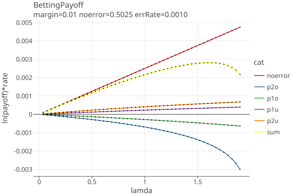
The sum of terms is the yellow line. The optimizer finds the value of lamda where eq 1 is at a maximum. Equation 1 is used just for finding the optimal lamda; the value of the equation is not used.
If there are no negetive terms or the negetive terms are not large (eg if p2o = 0), then eq 1 is monotonically increasing, and lamda will always be the maximum value allowed.
Betting with OneAudit pools
OneAudit cards are a mixture of CVRs and pooled data. The CVRS are handled exactly as CLCA above. Pooled data do not have CVRS, instead we have the average assort value in each pool.
Consider a single pool and assorter a, with upper bound u and avg assort value in the pool = poolAvg. The poolAvg is used for cvr_assort, so the overstatement error = cvr_assort - mvr_assort has one of 3 possible values:
poolAvg - [0, .5, u] = [poolAvg, poolAvg -.5, poolAvg - u] for mvr loser, other and winner
then bassort = (1-o/u)/(2-v/u) has one of 3 possible values:
bassort = [1-poolAvg/u, 1 - (poolAvg -.5)/u, 1 - (poolAvg - u)/u] * noerror
bassort = [1-poolAvg/u, (u - poolAvg + .5)/u, (2u - poolAvg)/u] * noerror
For each pool, we know the expected number of loser, winner, and other votes over all the cards in the pool:
    winnerVotes = votes[assorter.winner()]
    loserVotes = votes[assorter.loser()]
    otherVotes = pool.ncards() - winnerVotes - loserVotes
The expected rates are the votes divided by Npop. These are also the probabilities of drawing a card from that pool with that assort value.
Then we extend equation 1 with the expected assort values from the pools:
log T_i = ln(1.0 + lamda * (noerror - mui)) * p0 + Sum { ln(1.0 + lamda * (a_k - mui)) * p_k, k=1..n }
          + Sum { ln(1.0 + lamda * (a_pk - mui)) * p_pk; over pools and pool types}              (eq 2)

where
    p0 is the probability of no error (mvr matches the cvr)
    p_k is the probability of error type k
    a_k is the value of x when error type k occurs
    p_pk is the probability of getting pool p, type k
    a_pk is the assort value when pool p, type k occurs (k = winner, loser, other)
And use this to find the optimal value of lambda.
Compare Current OneAuditNoErrors with previous OneAudit plots to see the improvement using eq 2.
Estimating samples needed for OneAudit when there are no errors
The a_pk and p_pk values for OneAudit (eq 2 above) are known in advance, and do not need to be updated as we sample. We can estimate the number of samples needed for OneAudit when there are no errors in the CVR data, assuming an approximate µ_i = .5 and a constant bet of λc:
T_i = Prod (payoff_i, i= 1..i)
over N trials, there will be N * p terms, where p is the probability of that term:
T_n = (1 + λc (noerror − .5)) ^ (N*p0) * Prod { (1 + λc * (a_pk - 0.5)) ^ (N*p_pk) } = (1/alpha)

N * ln(1 + λc (noerror − .5))*p0 + N * Sum( ln(1 + λc (a_pk − .5)*p_pk) = ln(1/alpha)
N = ln(1/alpha) / (ln(1 + λc (noerror − .5))*p0 + Sum( ln(1 + λc (a_pk − .5)*p_pk))     (eq 3)
where p0 = 1 - Sum (p_pk), and λc is taken as the optimal value using eq 2 when all error probabilities are 0.
This value of N estimates the mean of a distribution that has a fairly large variance.
Suppose we have a OneAudit with one pool with 5% of the votes, and both the pool margin and the election margin are 2%, and there are no errors at all in the CVRs. The terms in equation 2 are:
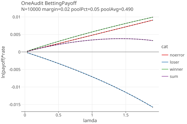
In this example, the optimal lamda is around 1.4. As the percent of cards in OneAudit pools increase, the negetive terms get large enough to curve the sum downward, then we get an optimal bet less than maxBet, and we need many more samples than CLCA without pools. Errors in the CVRs magnify the downward curve. A combination of small margin, large pool percentage and CVR errors will force the audit to a full hand count.
TODO: can we detect when a OneAudit will always go to a full hand count even without CVR errors, based only on the margin and the pool averages? We can see when eq 3 goes negetive, which I think means on average the OneAudit will go to a hand count, but the large variance allows the possibility that it will stop short of a full count. OTOH we can probably use the calculated variance to estimate the probability of a full count.
Choosing MaxLoss
MaxLoss is a user settable parameter which limits the maximum bet that can be placed on any one sample (see stalled audits).
How many noerror samples are needed to offset an assort value of 0.0, ie a 2-vote overstatement error (p2o) ?
The payoff for the jth bet:
tj = 1 + λ_j * (x_j − µ_j) (approximate µ_i as 0.5)
A p2o assort value of x = 0.0, gives the smallest possible value of tj:
tj = 1 + λ_j * (x_i − µ_j)
tj = 1 + λ_j * (0 − .5)
tj = 1 - λ_j / 2
Which is smallest when λ_j = maxBet = 2 * maxLoss
t_min = 1 - maxBet /2
t_min = 1 - maxLoss
which is how we choose maxLoss: whats the largest loss we are willing to suffer on a single sample? If maxLoss = .9, then t_p2o = .1, and we lose 90% of our “winnings” (aka the testStatistic T).
To compensate for one p2o sample at the maximum bet, we need n_p2o noerror samples, such that
payoff_noerror^n_p2o * payoff_p2o = 1.0
where
payoff_noerror = 1 + maxBet * (noerror − 0.5)
payoff_p2o = = 1 - maxBet /2
so
n_p2o = -ln(payoff_p2o) / ln(payoff_noerror)
n_p2o = -ln(1 - maxBet/2) / ln(1 + maxBet * (noerror − 0.5))
(see The effects of CLCA Errors for the general case).
payoff_noerror^ncomp = 1 / (1 - maxLoss)
ncomp = -ln(1 - maxLoss) / ln(1 + maxLoss * (v/(2-v)))
If there are no p2o samples, then the number of noerror samples we need to reject the null hypothesis is
payoff_noerror^n = 1 / alpha
n = -ln(alpha) / ln(1 + maxLoss * (v/(2-v)))
Ignoring other types of errors, the number of samples needed when there are k p2o errors are:
nsamples = n + k * n_p2o
Here is a plot of nsamples for values of k (0 .. 5) and two different margins v = .01 and .05:
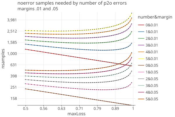
- When k > 0 there is a value of maxLoss that minimizes the number of samples needed.
- Informally you can see that the optimal maxLoss is the same for both margins. (click on the image to get an interactive html plot)
- This optimal maxLoss is probably the same value of optimalBet from our GeneralAdaptiveBetting function if there are no other errors, so we are already adapting to the error rates as we measure them. (TODO: check this)
- The optimal value of lamda varies by margin and error rates, but by setting the overall maximum loss to 0.9, we cut off possible increased sample sizes to the right of that.
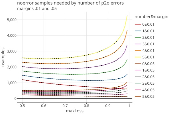
- The presence of even a single p2o error has a strong effect on the samples needed. The linear plot shows that more clearly:
Reducing maxLoss causes the ratio optimal/needed to be reduced by approximately the same percent (or less), as this table shows. Note the table also shows assort upper > 1 and < 1, as well as equaling 1.
maxLoss: 0.9000 N=100000, margin=0.01, upper=10.0 noerror:0.5003 maxtj: 1.0005: needed 6439 samples; pct = 0.9031
maxLoss: 0.9500 N=100000, margin=0.01, upper=10.0 noerror:0.5003 maxtj: 1.0005: needed 6111 samples; pct = 0.9516
maxLoss: 0.9900 N=100000, margin=0.01, upper=10.0 noerror:0.5003 maxtj: 1.0005: needed 5871 samples; pct = 0.9905
maxLoss: 0.9990 N=100000, margin=0.01, upper=10.0 noerror:0.5003 maxtj: 1.0005: needed 5820 samples; pct = 0.9991
maxLoss: 0.9999 N=100000, margin=0.01, upper=10.0 noerror:0.5003 maxtj: 1.0005: needed 5815 samples; pct = 1.0000
maxLoss: 1.0000 N=100000, margin=0.01, upper=10.0 noerror:0.5003 maxtj: 1.0005: needed 5815 samples; pct = 1.0000

maxLoss: 0.9000 N=100000, margin=0.01, upper=1.0 noerror:0.5025 maxtj: 1.0045: needed 662 samples; pct = 0.9003
maxLoss: 0.9500 N=100000, margin=0.01, upper=1.0 noerror:0.5025 maxtj: 1.0048: needed 628 samples; pct = 0.9490
maxLoss: 0.9900 N=100000, margin=0.01, upper=1.0 noerror:0.5025 maxtj: 1.0050: needed 602 samples; pct = 0.9900
maxLoss: 0.9990 N=100000, margin=0.01, upper=1.0 noerror:0.5025 maxtj: 1.0050: needed 597 samples; pct = 0.9983
maxLoss: 0.9999 N=100000, margin=0.01, upper=1.0 noerror:0.5025 maxtj: 1.0050: needed 596 samples; pct = 1.0000
maxLoss: 1.0000 N=100000, margin=0.01, upper=1.0 noerror:0.5025 maxtj: 1.0050: needed 596 samples; pct = 1.0000

maxLoss: 0.9000 N=100000, margin=0.01, upper=0.67 noerror:0.5038 maxtj: 1.0068: needed 444 samples; pct = 0.9009
maxLoss: 0.9500 N=100000, margin=0.01, upper=0.67 noerror:0.5038 maxtj: 1.0071: needed 421 samples; pct = 0.9501
maxLoss: 0.9900 N=100000, margin=0.01, upper=0.67 noerror:0.5038 maxtj: 1.0074: needed 404 samples; pct = 0.9901
maxLoss: 0.9990 N=100000, margin=0.01, upper=0.67 noerror:0.5038 maxtj: 1.0075: needed 400 samples; pct = 1.0000
maxLoss: 0.9999 N=100000, margin=0.01, upper=0.67 noerror:0.5038 maxtj: 1.0075: needed 400 samples; pct = 1.0000
maxLoss: 1.0000 N=100000, margin=0.01, upper=0.67 noerror:0.5038 maxtj: 1.0075: needed 400 samples; pct = 1.0000